Introduction

• This demo script demonstrates how to visualize the Spatial Omics Set (soSet) to facilitate interpretation of the derived metagene structure and cross-cohort relationships.
• Each figure generated below is accompanied by a detailed explanation describing its rationale, key features, and guidance for interpretation.

Directory settings

• This block defines the working directory used throughout the demo to store downloaded inputs and generated outputs.

# If you want to use a user-defined output directory, 
# uncomment and set the download_dir parameter.

# download_dir <- "/path/to/download" # where soObj.RDS is located

if (exists("download_dir") && is.character(download_dir) && length(download_dir) == 1 && 
        nzchar(download_dir)) {
        download_dir <- download_dir
} else {
        download_dir <- tools::R_user_dir("sotk2", "data")
}

Load the spatial omics object

• We load the previously generated soObj object, which contains the correlation network and community detection results produced in the earlier steps of the workflow.
• The script first attaches the sotk2 package and then checks whether soObj.RDS is present in download_dir.

library(sotk2)

if (file.exists(file.path(download_dir, "soObj.RDS"))) {
        soObj <- readRDS(file.path(download_dir, "soObj.RDS"))
} else {
        stop("ERROR: the soObj.RDS file not found.")
}

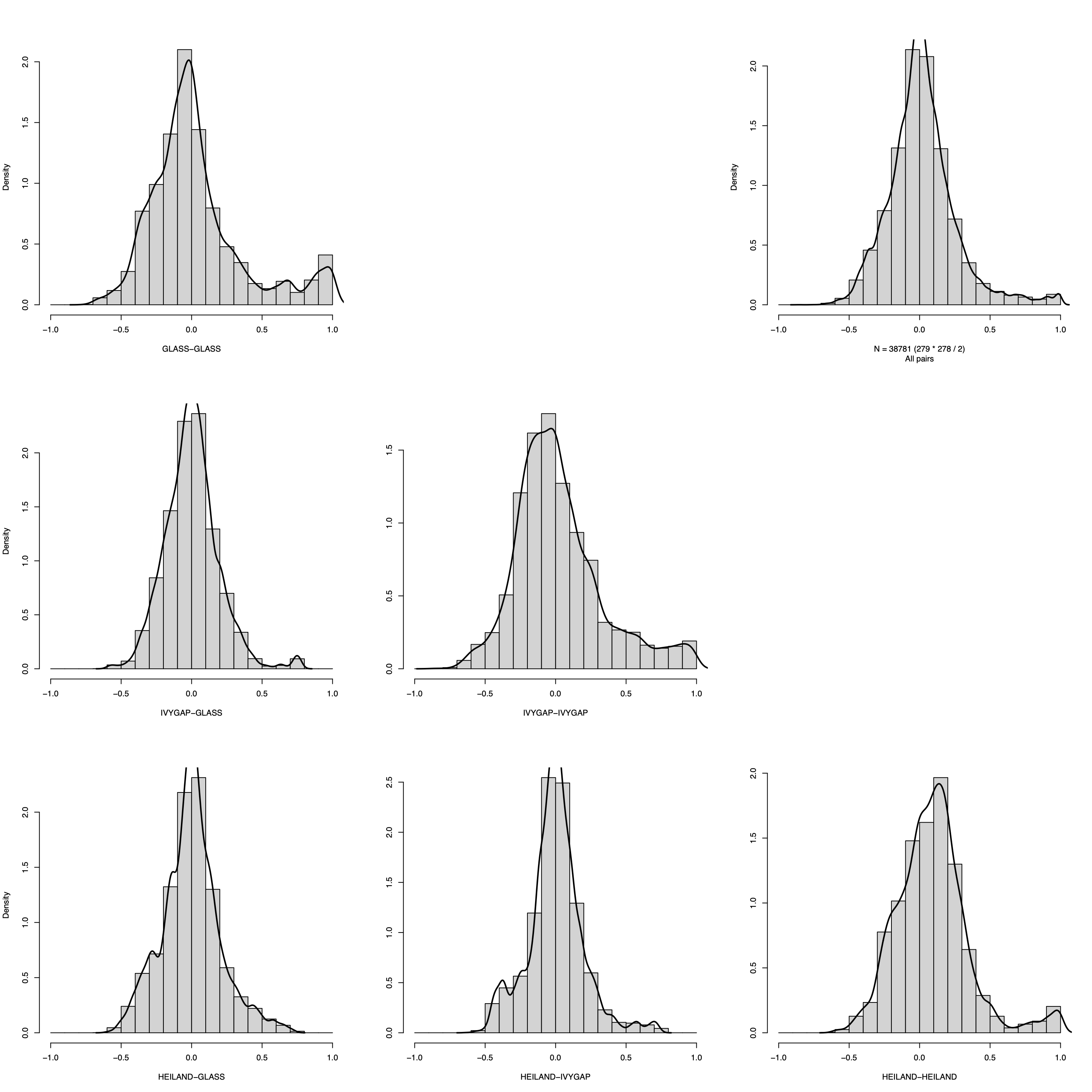
Correlation coefficient density

• This panel summarizes the distribution of pairwise correlation coefficients within and between datasets using a matrix-style layout.
• For three datasets, the figure comprises six histograms corresponding to all dataset pairs.
  1. The diagonal panels display within-dataset correlation distributions.
  2. The lower-left panels show between-dataset correlation distributions for each dataset pair, whereas the upper-right panels provide the corresponding overall coefficient distributions as a reference for comparison.
• The filename argument controls output: setting filename = NULL prints to the active graphics device, whereas providing a path writes the figure to disk.

plotCorrDensity(soObj@SOSet, filename = NULL)

Visualization parameters

• This section defines core visualization parameters that control the appearance and readability of the network plots.
• Specifically, nodeSize and nodeLabelSize determine the size of nodes and the corresponding label text, respectively, while edgeAlpha sets the transparency of edges to reduce visual clutter in dense networks and to emphasize higher-level structure.

nodeSize        <- 10
nodeLabelSize   <- 2
edgeAlpha       <- 0.8

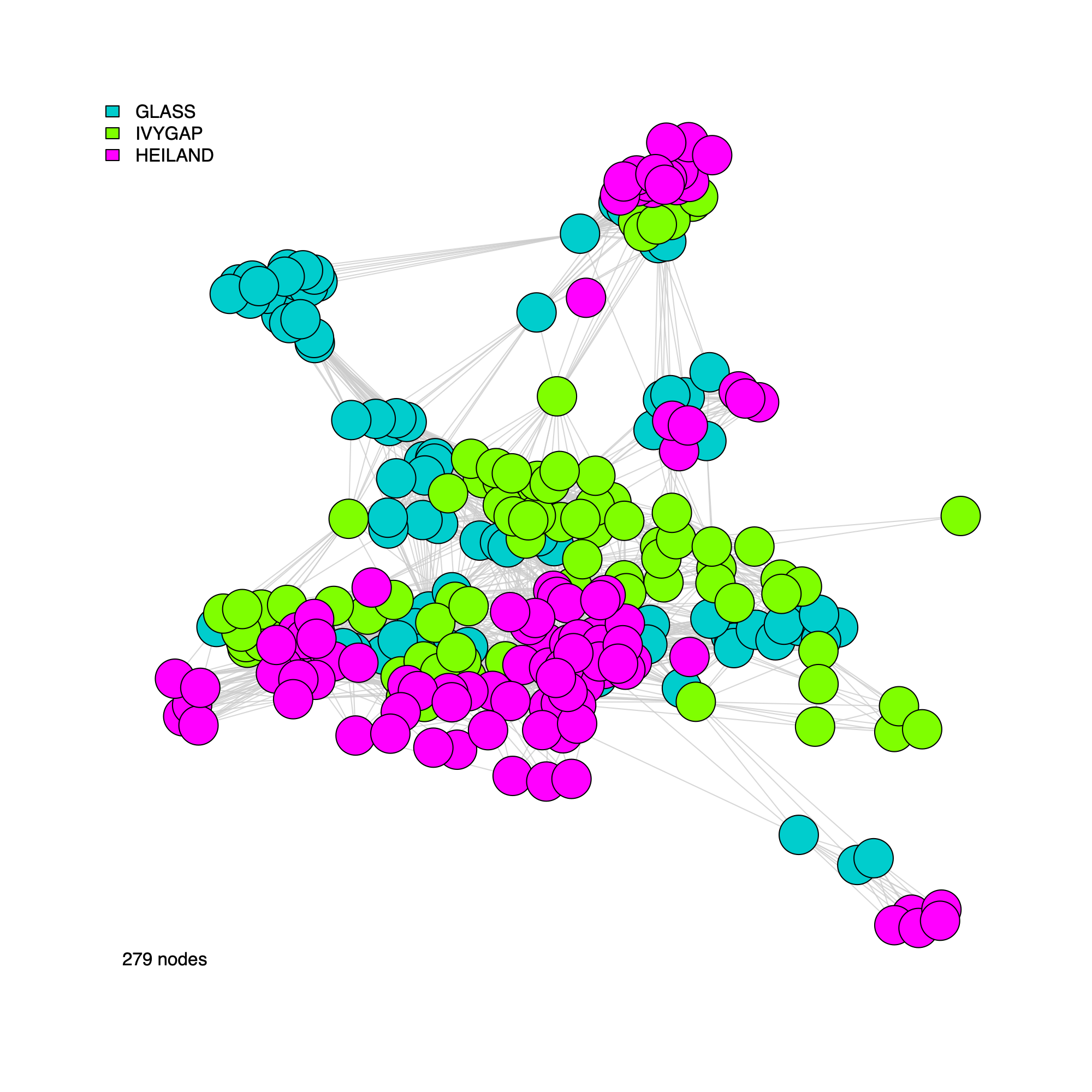
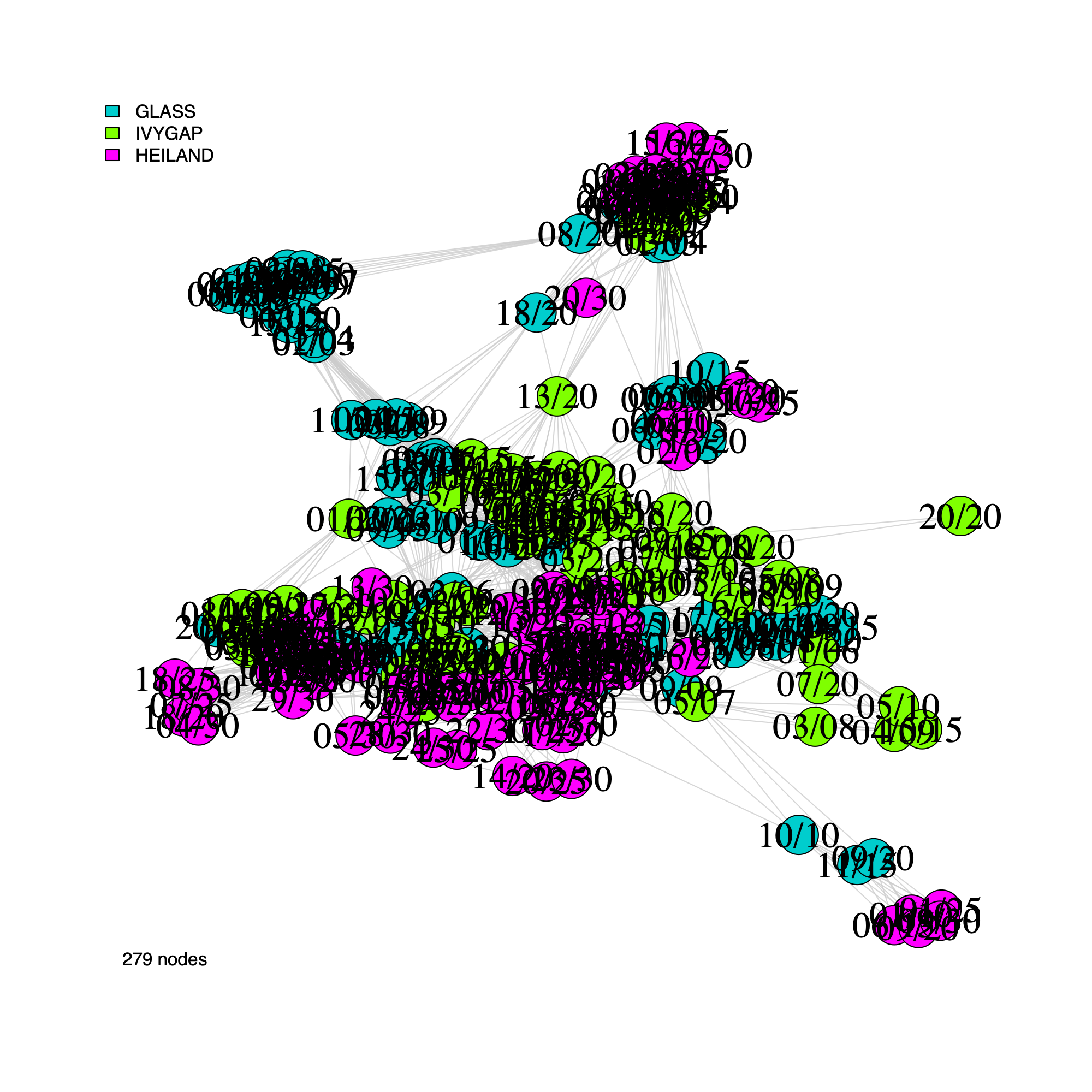
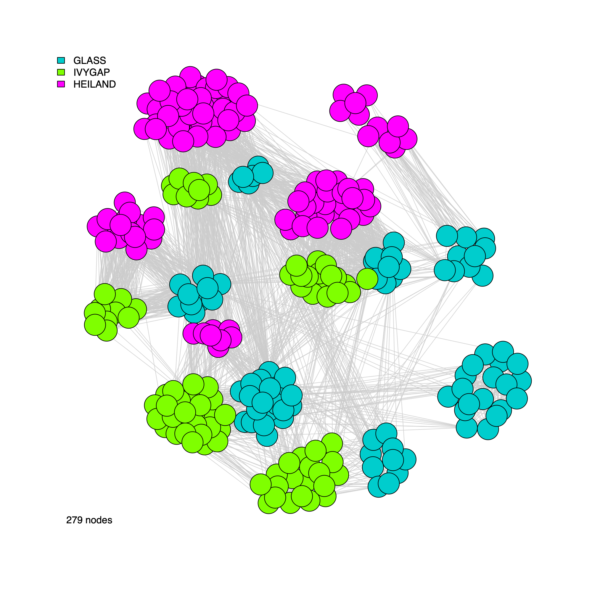
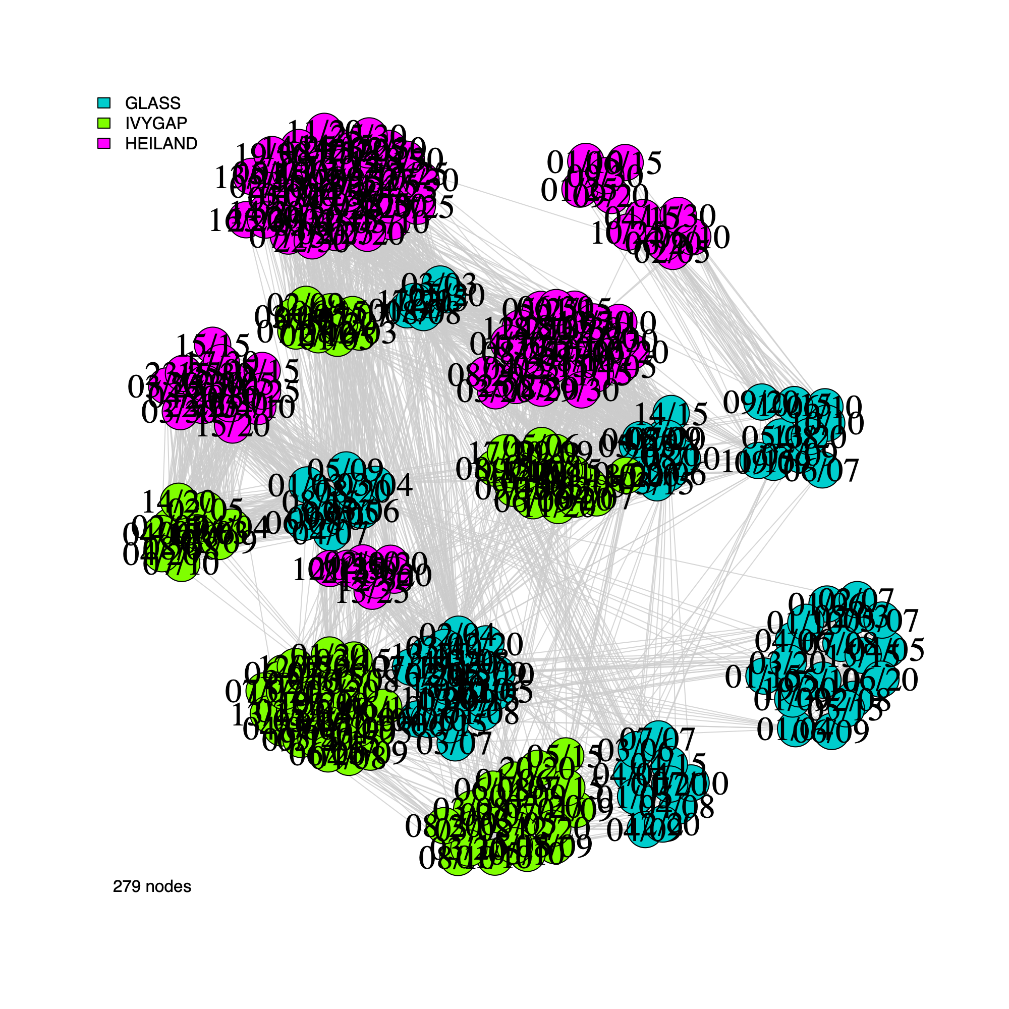
Correlation-network plots

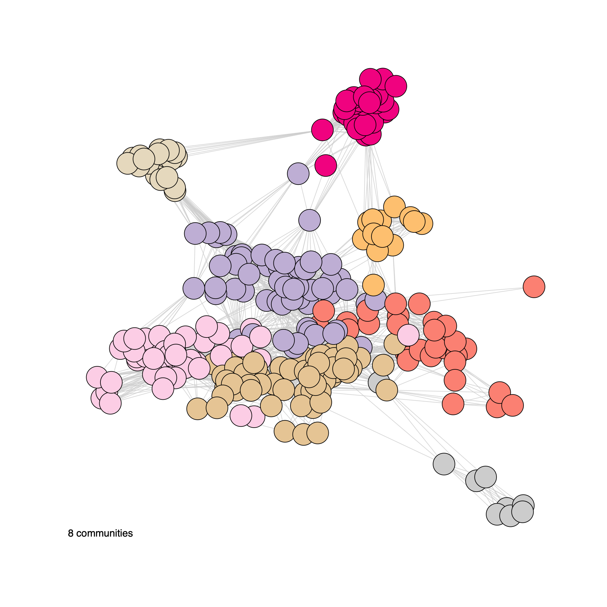
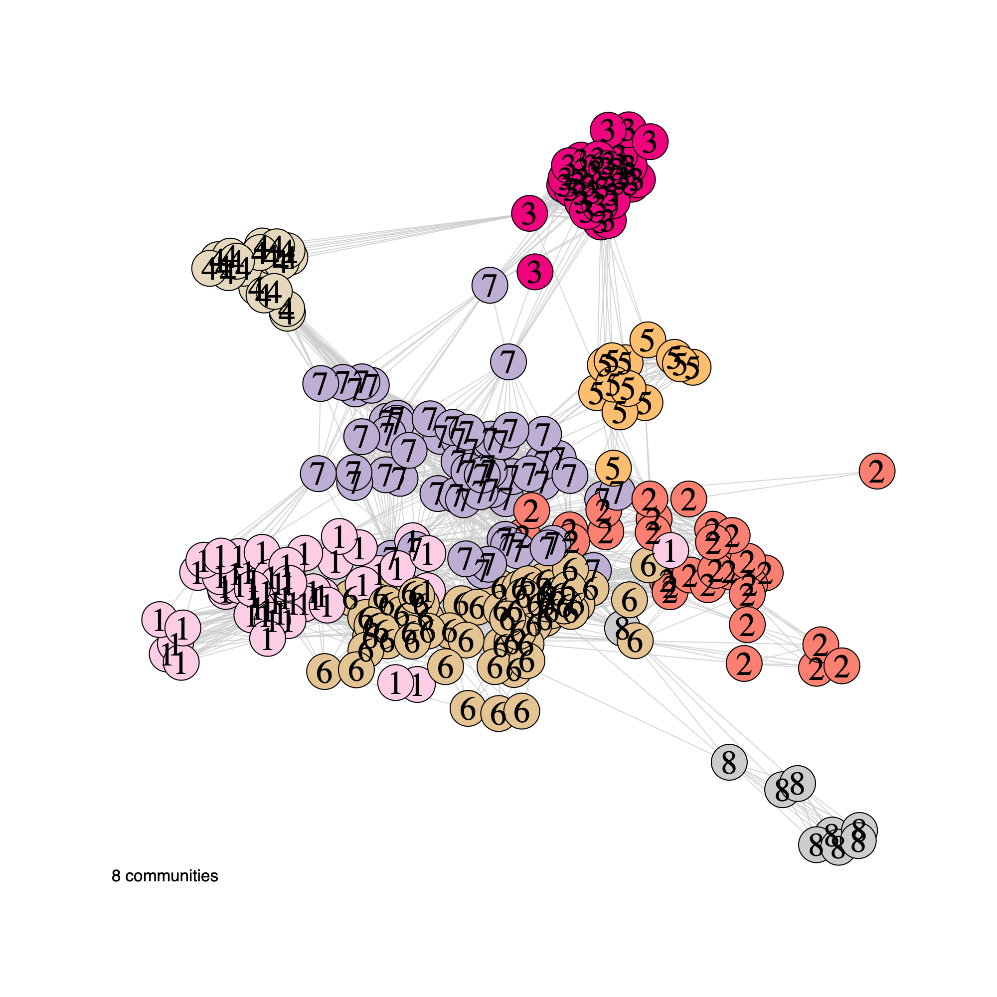
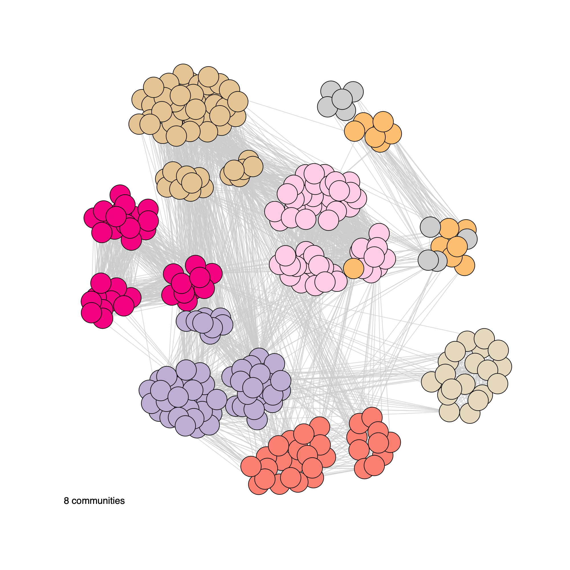
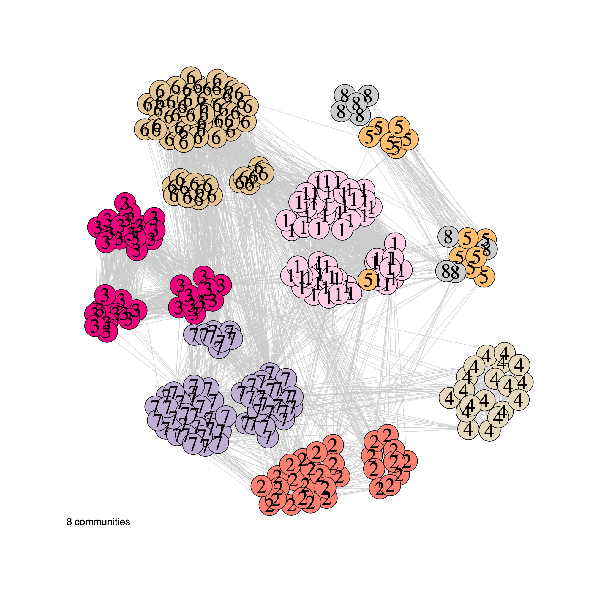
• In this section, we generate network visualizations derived from the correlation graph stored in soObj.
• The plotting function supports flexible display options, allowing users to
• Toggle vertex labels (label = TRUE/FALSE)
• Color or annotate nodes by cohort membership (annot = "cohort") or by inferred community assignment (annot = "community")
• Render either an unweighted network (weighted = FALSE) or a weighted network (weighted = TRUE, where edge widths reflect correlation strength)

plotNetwork(soObj, label = FALSE, annot = "cohort", weighted = FALSE, edgeAlpha = edgeAlpha, filename = NULL, vertexSize = nodeSize, vertexLabelCex = nodeLabelSize)

plotNetwork(soObj, label = TRUE, annot = "cohort", weighted = FALSE, edgeAlpha = edgeAlpha, filename = NULL, vertexSize = nodeSize, vertexLabelCex = nodeLabelSize) 

plotNetwork(soObj, label = FALSE, annot = "community", weighted = FALSE, edgeAlpha = edgeAlpha, filename = NULL, vertexSize = nodeSize, vertexLabelCex = nodeLabelSize)

plotNetwork(soObj, label = TRUE, annot = "community", weighted = FALSE, edgeAlpha = edgeAlpha, filename = NULL, vertexSize = nodeSize, vertexLabelCex = nodeLabelSize)

plotNetwork(soObj, label = FALSE, annot = "community", weighted = TRUE, edgeAlpha = edgeAlpha, filename = NULL, vertexSize = nodeSize, vertexLabelCex = nodeLabelSize)

plotNetwork(soObj, label = TRUE, annot = "community", weighted = TRUE, edgeAlpha = edgeAlpha, filename = NULL, vertexSize = nodeSize, vertexLabelCex = nodeLabelSize)

plotNetwork(soObj, label = FALSE, annot = "cohort", weighted = TRUE, edgeAlpha = edgeAlpha, filename = NULL, vertexSize = nodeSize, vertexLabelCex = nodeLabelSize)

plotNetwork(soObj, label = TRUE, annot = "cohort", weighted = TRUE, edgeAlpha = edgeAlpha, filename = NULL, vertexSize = nodeSize, vertexLabelCex = nodeLabelSize)

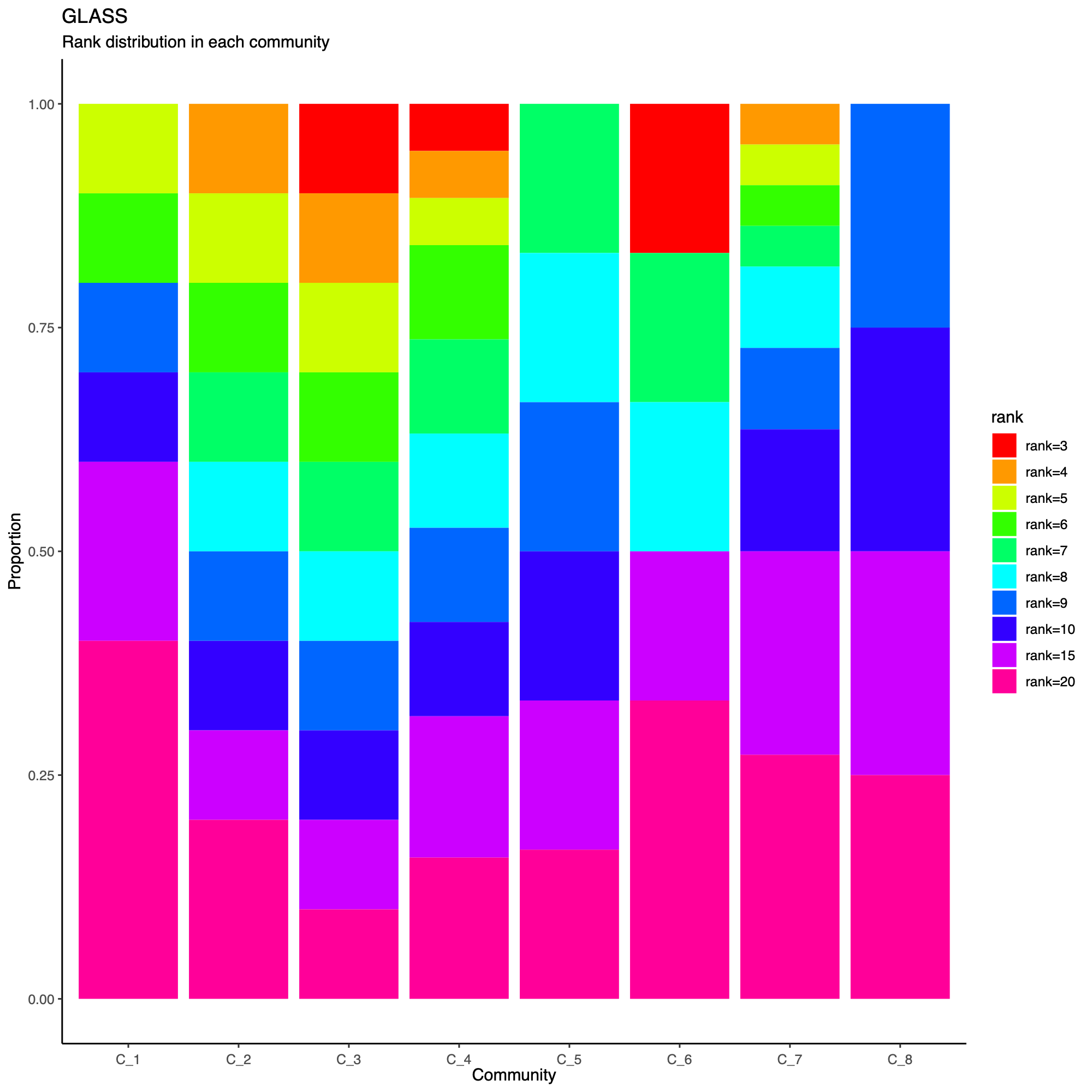
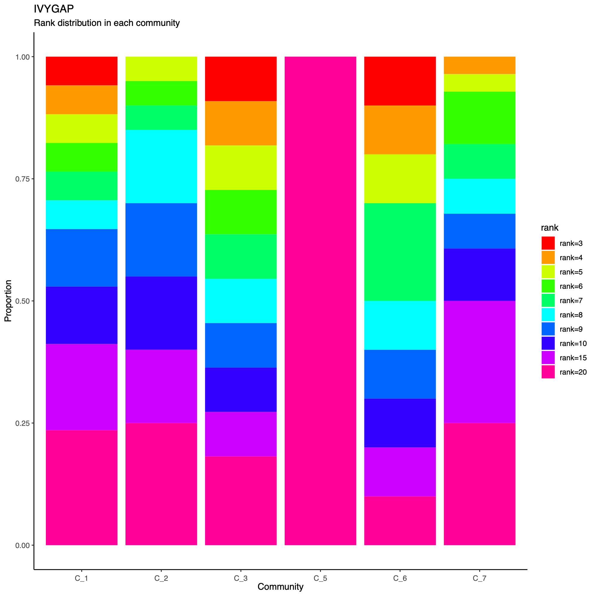
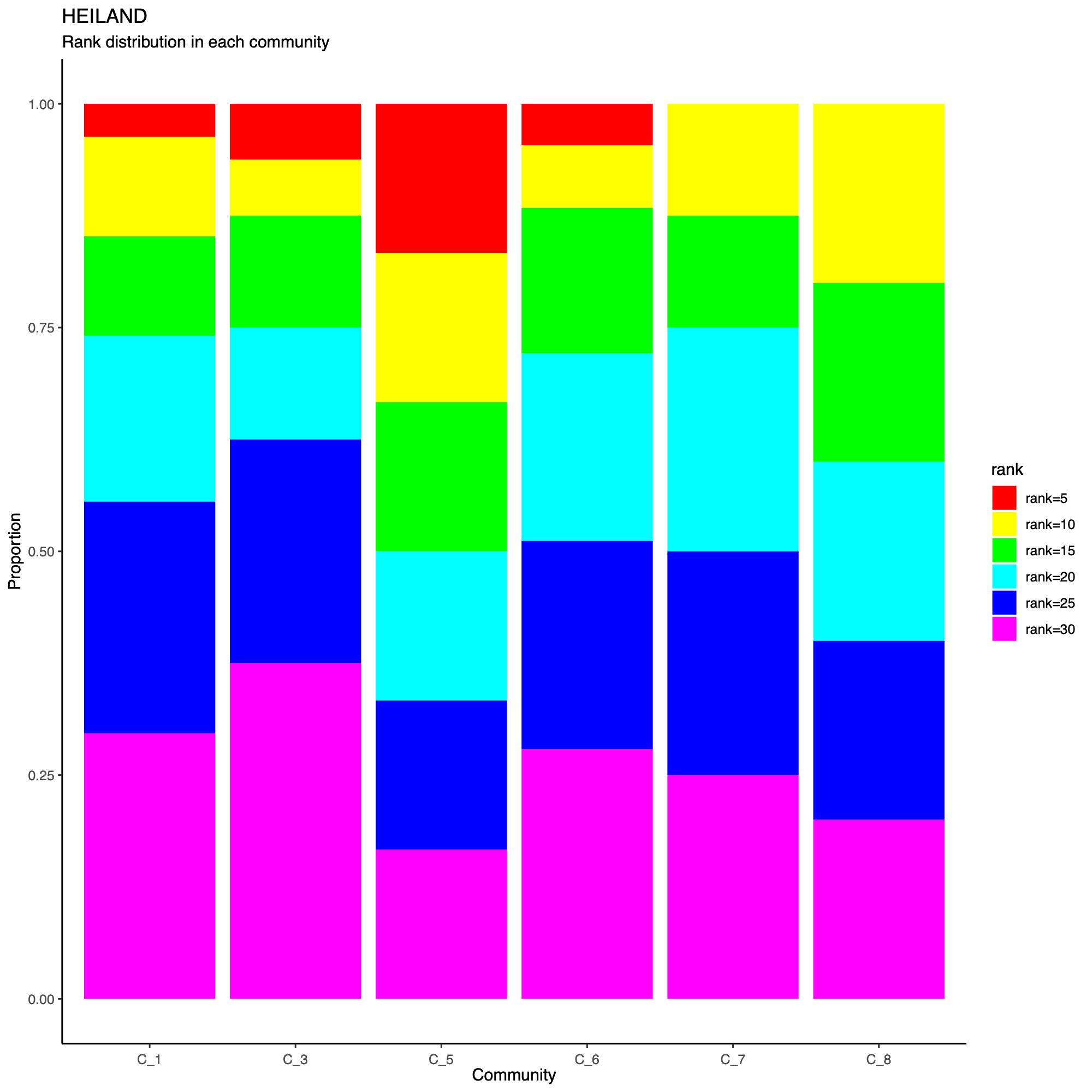
Community network properties

• The following plot summarizes community composition by reporting the number of metagenes assigned to each detected community, stratified by dataset.
  1. This visualization provides a compact overview of how communities are supported across cohorts and highlights communities that are cohort-specific versus broadly shared.
  2. Metagenes derived from higher-rank factorizations often capture increasingly sample-specific patterns rather than broadly conserved biological programs. Consequently, communities dominated by high-rank metagenes may reflect cohort- or sample-idiosyncratic structure and may be less likely to represent generalizable biological signals that are reproducibly observed across datasets.

statComm(soObj, filename = NULL)

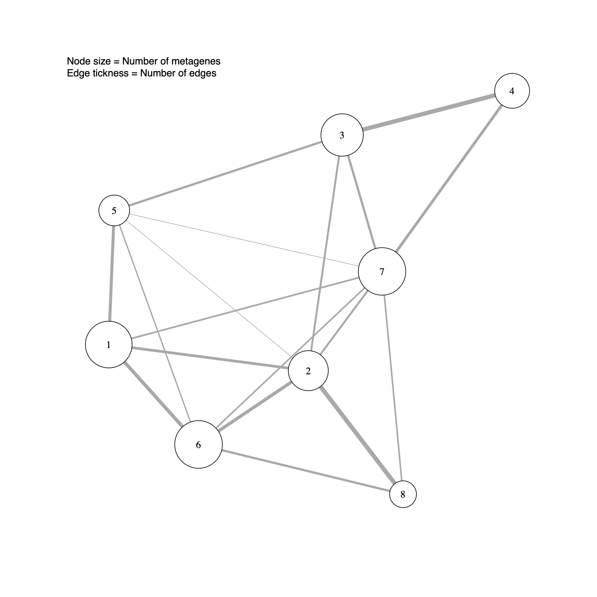
Community-level network layout

• This step generates a community-level network in which each node represents a detected community.
• Node size reflects the number of metagenes (GEPs) assigned to the community, and edge thickness summarizes the extent of connectivity between communities (that is, the number of inter-community edges in the underlying metagene network).
• In subsequent sections, this community-level layout will be augmented with sample-level annotations to support biological interpretation of the inferred modules.

plotCommNetwork(soObj, vertexInfo = NULL, filename = NULL)